 Zeepabyte
Zeepabyte
Cascade Analytics System demonstrated outstanding performance during Star Schema Benchmark tests at Mellanox Technologies Labs while using minimal computing resources and power.
Single node
600 mln rows
qph@SF
3 nodes
600 mln rows
qph@SF
4 nodes
1.8 bln rows
qph@SF
5 node
6 bln rows
qph@SF
Star Schema Benchmark is similar to TPC-H benchmark and uses the same performance metrics. The charts below compare Cascade results with current TPC-H leaders.
(qph@SF)
performance per node
Performance per CPU core
Cascade's cost of performance is about 10x lower compared to the leaders in TPC-H.
See complete benchmark report here.
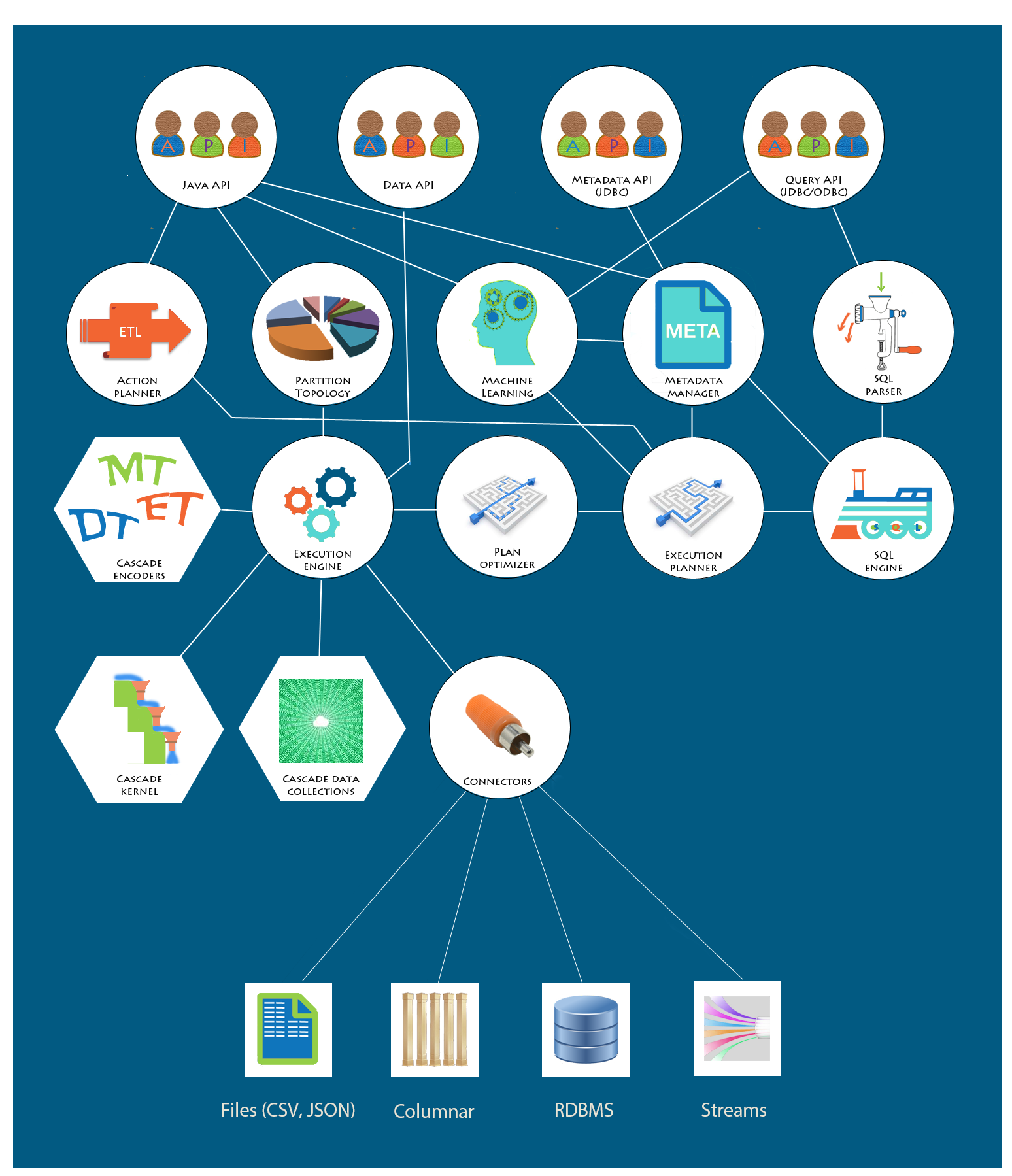
Cascade Analytics System handles a variety of analytic tasks in a variety of environments. Cascade efficiently runs execution plans arising from queries, ETL, machine learning tasks, etc.
Cascade can run on a single node or on a cluster, in-memory or disk-based. It is not dependent on any specific distributed computing environment, as long as it can use the environment's RPC (Remote Procedure Call) mechanism. It can run on Hadoop if necessary, taking advantage of its features, but it can also run using its own capabilities based on Apache Thrift RPC mechanism. This mechanism was used during the Star Schema Benchmark tests.
Any logical node can run some number of services, such as JDBC query and JDBC metadata services and data services. A physical node can run several logical node processes, attached to a different TCP/IP port. Default port for Cascade logical node services is 8989. Besides, one logical node must play the role of metadata reconciliator, i.e. it makes sure that all encoding dictionaries are reconciled.
Zeepabyte technology is based on unique multidimensional indexing techniques. Database technologies have a long history of evolution. Recent trends lead towards specialization of databases rather than attempting to produce a single answer to all challenges and workloads. "One size fits all?" lecture by Michael Stonebraker, MIT professor and well-known database expert, set start to a number of initiatives.
In the analytics domain, columnar data organization became popular because it addressed the requirements of the analytic workloads better than row storage. Columnar organization allows compressing data better and fitting more data into memory. However without indexing, answering a query still requires a full scan of all the data records. Traditional indexing remains expensive; it takes time and space. Analytic workloads usually require combining several individual column indices to obtain an answer to a query, and the number of combinations of columns involved in queries may be huge.
Data which must be analyzed originates from certain business processes, such as sales of goods, mobile phone calls, messaging, Internet access, industrial sensor data, etc. Business requirements yield assigning roles, such as dimensions, to attributes that drive the business process whose data is captured in a data warehouse. Cascade Analytics System stores data from multiple dimensional attributes directly in its "cascade" data structure that also serves as an index. Other attributes, playing measure roles, can be stored in columns for efficiency. But most of the business questions restrict one or more dimensional attributes, and the "cascade" data structure plays a central role.
Such data organization can be considered as creating a single "composite key" column in addition to measure columns. But that column is also itself a multidimensional index that allows fast filtering by any combination of point, range and set constraints. At the same time it ensures a much higher level of compression than columnar storage. Data ingestion rates are also higher because only one index is built rather than an index per dimension. Finally, "cascade" uses no additional storage for the index itself. No decompression is necessary for processing the majority of the queries, until the result is presented for the end user. Thus the data in the "cascade" structure in memory and on disk is not human readable which ensures additional security.
Years of research and practice with multidimensional indexing techniques by Zeepabyte founders Dr. Alex Russakovsky and Ram Velury went into inventing the patent pending techniques behind Cascade. The World record performance of Cascade in Star Schema Benchmark confirms the efficiency of this approach.
In a typical usage scenario, after the system is configured and started, and the necessary metadata is created, users start submitting analytic tasks. The tasks can be predefined once and executed at certain moments, driven by either timer or data events (stream-like configuration), or they can be user or application-driven ad-hoc queries or machine learning scoring requests.
Examples of predefined tasks are data ingestion, materialized view maintenance, machine learning processes, monitoring, alerting, etc. It is very important to be able to do all this faster than the data comes in, and Cascade can support high data input rates.
Examples of ad-hoc tasks are queries, user-driven data exploration, scoring against machine learning models, recommendation systems, etc. If queries pose a significant number of point, range or set constraints, Cascade technology ensures real time response times, even with limited resources, on billions of data records.
Today's functionality focuses on ad-hoc queries, and the present description explains it in the context of the Star Schema Benchmark. For those who wish to get started right away can take a look at a simple "Hello, world!" application.


Cascade implementation is based on MPP (Massively Parallel Processing) principles, with data typically distributed over partitions residing on several cluster nodes. Each of the partitions has data split into keys and values (dimensions and measures). Keys are organized into "cascade" index structure which is highly compressed and usually entirely fits in memory. Measures can reside in memory or on disk and are typically organized into columnar storage. If necessary, additional indices can be created on those columns, as in columnar databases. But for the Star Schema Benchmark, no additional indices were necessary.
During query processing, each partition is processed independently of the others. This ensures a high level of parallelism, and the results are combined as they become available. Cascade features multiple kinds of data collections that hold intermediate results during partition processing. These collections are also fast and easy to combine.
When a query comes in through SQL interface, such as JDBC, it is parsed and reworked into an initial execution plan using metadata repository to resolve context and variable names. The plan is then optimized by Cascade optimizer and given to the Execution engine for execution. When several nodes are involved, the plan is automatically split into local and remote plans. If several partitions need to be processed, the plan is distributed to those partitions. More information about the execution plans can be found below.
The instance of Cascade that runs on the query origination node (query node) executes the local portion of the plan and delegates remote plans to remote data nodes using appropriate Remote Procedure Call (RPC) mechanism. The query node can serve as a data node itself. Cascade is not tied to a specific RPC mechanism, and can use its own, Apache Thrift based, mechanism or use e.g. Hadoop RPC mechanisms (typically through HBase coprocessor mechanisms, although HBase is not used for data storage).
Data load into "cascade" data structure requires the dimensional data to be encoded. Encoding setup can be a separate step in the data load process or can be combined with actual load of data into "cascade". A component called Action Planner decides how to organize the ETL process and creates either two execution plans - one that generates encoders and one for data load - or combines them into one. Execution plans originating from ETL can be quite complex, because some encoders can be created in parallel, while some may have to be created after the others.
Encoder data is stored on disk but is kept in memory at all times; it is usually very small. Encoders can be Master Tables (dictionaries), Dependency Tables, or Equivalence Tables (the term table does not signify how encoders are organized but reflects the fact that they may be queried as tables). "Cascade" data sets are also persisted, so that they do not need to be rebuilt upon system restart. However they can be configured to be completely transient. Both encoders and data sets support bulk updates rather than individual transactions.
Data from external sources can be read with the help of connectors. Readers can find more information about connectors elsewhere on this site. Connectors for CSV files and relational databases such as MySQL or SQL Server are available with Cascade. Some other connectors may be built on demand.
Cascade serves as a Business Intelligence (BI) system which means that it can execute queries or machine learning tasks against all its data sources without moving the data in. To some data sources, such as RDBMS, parts of such tasks may be delegated, some other sources, like files, are processed by the appropriate connectors and specific algorithms. Efficiency of execution is limited by the abilities of the data source.
Cascade Analytic System can organize data into its highly efficient internal data structure, Cascade data set. This structure features a highly compressed multidimensional index capable of exceptional performance due to ability of the engine to avoid full scan on queries with filters. As is evident from Star Schema Benchmark results, Cascade data sets ensure significantly better performance than any other presently known database product, often by orders of magnitude, on workloads consisting of ad-hoc queries with dimensional constraints. Besides, there is no "index building" process: the data is loaded directly into the index with high ingestion rates allowing Cascade to organize data streams into data sets immediately available for querying in real time.
As an analytic database, Cascade supports bulk loads into data sets rather than individual transactions. Data transformations necessary for data load (ETL) are in most cases automatically designed, transformed into an execution plan by Cascade's Action Planner, and executed by Cascade's execution engine. Design procedure takes advantage of metadata declarations provided by the user and supports many normalized and denormalized source data organization kinds, in particular denormalized fact tables, star and snowflake schemas, etc. Additional transformations may be also directly inserted into the plan by the user. Read more about execution plans below.
A simple "flat" record is a tuple (vector) of data whose components represent values of supported data types. Records usually represent events in some business process, such as sales events in which a customer is buying products at some store. Customer, product, store, transaction time, price paid, etc., are components of the records. More complex records may have other records as components ("nested records").
A data type is a descriptor of the functional properties of a value, such as internal representation, conversions, serialization, orderings, etc. Cascade supports at least the following data types:
There is a correspondence between Cascade data types and SQL data types. Cascade has the ability to perform the necessary transformations for consuming SQL DDL or for JDBC metadata exploration interface.
Expressions operate on values. An expression can take one or more values of the above mentioned types and return some other value, e.g. a + b; Cascade supports functions and operators commonly used in SQL and supports extension by user defined functions.
A tuple of expressions can be used to transform a record of arguments into a record of result values. This is an example of a record operation.
Operations performed by Cascade on records during execution usually fall into two categories: record and window transformations.
A record operation transforms a record of data without taking other records into account. Example: select a subset of record components, calculate an expression formulated in terms of record components, etc.
A window operation requires accumulating some set ("window") of records to transform them. Example: sorting records, aggregating, matrix inversion, pivoting, etc.
A logical transformation represents an abstraction (descriptor) for record and window operations. Logical transformations are used when a logical execution plan is created and optimized. A logical plan can be then converted into an executable plan. During conversion, some of the logical transformations are replaced with executable transformations, some are delegated to specialized data collections, and some are turned into flow control nodes of the execution plan.
Examples of transformations commonly used in data load and query scenarios can be found below:
Execution plan is a directed acyclic graph of execution nodes with node-specific edges. In a logical plan, nodes contain logical transformations. A single node may contain several record operations, but at most one window operation. Each node has one or more execution algorithms.
A node is a pass-through if all its operations are record operations. When a logical plan is converted to executable form, some of the node's logical transformations may be converted to executable transformation and some delegated to specialized internal data collection (see more about data collections in Metadata and deployment). A specialized collection can be sorting records or grouping them by some key, etc.
Some of the nodes are used for program flow control, i.e. they programmatically orchestrate execution of other nodes. Some other nodes have a combined responsibilities as both control and operations.
Commonly used types of nodes in Cascade execution plans are:
Cascade takes care itself of converting queries or ETL to execution plans, but client side Data API, due to appear soon, would allow programmatic user control over combining particular transformations into a plan and executing it.
Cascade Analytics System is a Business Intelligence (BI) system, and, according to common BI practices, both logical and physical elements of the schema must be defined. Queries are then formulated in terms of the logical elements while the underlying physical schema can seamlessly change without the need to change queries.
Cascade supports SQL for queries via JDBC and ODBC API. Thus Cascade Analytics System may function as an analytic database, and is capable of running the Star Schema Benchmark. However as an analytic database it supports only bulk data loads.
Cascade also supports JDBC metadata API, but not DDL via JDBC because Cascade metadata is richer than in a typical RDBMS.
Let us examine the metadata elements and the process of metadata authoring.
In a typical BI scenario, users are distinguished by their roles. For understanding Star Schema benchmark setup in Cascade, it is sufficient to consider two main categories of users.
Business experts (application designers) are those users who understand the driving forces of their business and express their declarations in terms of logical elements: business attributes, relationships and processes. They do not need to be familiar with details of data storage formats.
Data experts are those users who understand format and structure of specific sources of data, but not necessarily the semantics of their elements. They work on describing the physical organization of those sources and collaborate with business users on defining bindings between the logical and the physical elements of Cascade metadata. Bindings are expressions that define how to obtain values of a logical variable.
Logical schema is the heart of a BI system. Other categories of users, such as report and UI designers, can start their design work as soon as the logical schema is defined. However no data would flow to reports, dashboards and other UI elements until physical schema is in place, and bindings are defined.
Logical elements represent business objects with which business users deal as part of their business processes, such as Time, Part, Customer and Supplier in the case represented within the SSB scenario. Additionally, geographical attributes, such as City, Country and Region, classification attributes, such as Brand, Category or Group, etc. as well as relationships between attributes (business semantics) can be important for business analysis purposes.
Definitions of logical elements in Cascade Analytics System can include additional information such as possible ranges of values and declared statistics of both data distribution and usage. The more of such information provided upfront, the better Cascade can prepare for the planned workloads.
Physical elements represent details of specific data organization, for example, primary and foreign keys in normalized data sources - which typically have no specific business meaning. These elements may also engage in relationships, and the logic inside a BI system uses these relationships to infer proper data organization process and query resolution specifics. A typical internal usage consists in adding or removing joins between sources while processing a logical query.
Source is a metadata descriptor for an object from which data could be read, and sink is a metadata descriptor for an object to which data could be written. A metadata object can be a source and a sink at the same time.
Data collections are actual objects containing data. They can be readable or writable or both. Sources and sinks are metadata descriptors for them. The same source could potentially describe structure of multiple collections. However sources and sinks contain also certain "deployment" information, a set of details regarding partitioning, underlying data structure, persistence, etc. This deployment information is captured in an object called connector. Each connector type is uniquely defined by a protocol string.
Connectors are plug-ins in the system and can be easily added as needed. Several useful connectors are shipped with Cascade. This includes delimited files (such as csv or tsv, etc), generic JDBC connectors (with dialects for MySQL, Oracle, Postgres, SqlServer, etc) and connectors for internal Cascade data collections. A source or sink may be defined without any connector during design time, but would need connector to be defined before data operations.
Cascade source kinds are simple source, schema and star. Source is similar to a table in relational model, schema is collection of related sources (e.g. a fact table and related dimension tables) and star is a Cascade-organized schema, logically equivalent to some original schema. Star is also a sink, so that data can be written to the corresponding data collection.
As any BI system, which in essence is a federated database that can address queries to the original sources of data, Cascade is capable of serving such queries. However users have the opportunity to drastically improve performance of these queries by allowing Cascade to organize the data in its internal multidimensional format optimized for ad-hoc queries on a large number of attributes. The process of such data organization consists of two parts: data encoding design and actual data load.
Cascade's internal data representation assumes conversion of all values of certain attributes into integers (encoding). These integers are then used to create a composite key - another integer whose bits are a mixture of bits of the integers representing participating attributes. Details are covered elsewhere in Cascade documentation; for encoding design, the most important aspect is the following.
The objective of metadata definitions is to provide enough information to determine the number of bits necessary to allocate for all values of an attribute that will be encoded. In other words, Cascade needs to know the approximate cardinality of the attribute. Although this number can potentially change in the future, it is beneficial to have it reasonably defined upfront: make sure existing values and possibly expected updates are covered. Unused bits may be expensive.
If the attribute is Gender, we expect two values: "male" and "female". So we can suggest 2 as the cardinality. If we know that gender may be missing in the data ("null" value), we can declare it as 3. But no other updates are expected, so no need to declare higher cardinality.
Another example is Customer: today a business has 1 million users but expects that number to grow to 5 million within a short period of time. Although it costs 3 additional bits, it may be beneficial to declare cardinality as 5 million upfront. Only the next power of 2 matters, so such declaration would actually allow to handle growth up to about 8 million of users. There are other considerations involved in cardinality declarations as well.
An important example is Time (or Date). Multiple factors need to be taken into account: granularity of time measurement, data lifecycle (how long to keep the data and periodicity of updates), desired granularity in queries, etc. Fortunately, for Star Schema Benchmark, time setup is not very complex, but still requires careful handling.
Ways for Cascade to determine cardinality from metadata declarations:
The first 3 cases are obvious; in the last case the user is basically instructing Cascade to scan the source to which the binding can be referring. If this source is a dimension table in a Data Warehouse, determining the cardinality and designing the encoder takes insignificant time, but if binding is to a fact table, it may be very expensive. So even a rough upper bound approximation of the cardinality would be beneficial. Examples of all four kinds of declarations can be found in the Star Schema Benchmark definitions.
Internal Cascade data objects are encoders for attributes and relationships. There are two types of attribute encoders: dictionary based encoders (Master Tables) and transformation based encoders. Transformation based encoders encode values via certain expressions; Master Tables consult a dictionary (which is a data collection) for the encoded value. Similarly there are two types of relationship encoders: tabular (Dependency Tables and Equivalence Tables, which are data collections) and transformation based encoders. Relationships in Cascade are encoded if participating attributes are encoded. Encoders may be shared with other nodes in the system that run Query or Load services. They are persisted, so no need to rerun encoder creation unless there are updates to process. MT, DT and ET sources are available for querying but usually there is no need for the user to query them except for Master Data Management purposes. Of all these objects, only dictionaries are human readable, and they are stored separately from data for security purposes.
The following kinds of attributes are distinguished:
Logical and physical metadata elements (attributes and columns) can enter relationships which are important for analysis. The main ones are dependency relationships and equivalence relationships. Each relationship must have bindings to appropriate data in order for Cascade system to take advantage of it. An instance of a relationship is called a rule.
While attributes are global to the project, they enter into relationships within some context, hence rules must declared within the context of some source. The bindings for the rules must be to physical elements within that source.
Dependency rules establish functional dependency between attributes, e.g. that Country is a function of City (each City has only one Country), or between groups of attributes ("star rules"). The independent variables (first argument) of the star rule are often called dimensions; they would need to be encoded. If they also serve as independent variables of simple dependency rules (such as dependency between City and Country), we say that dimension has an associated hierarchy, and the dependent variables (second arguments) in those rules are called levels of the hierarchy. Some BI products call them dimensions as well. To avoid confusion, Cascade deliberately stays away from this terminology.
Equivalence rules establish a bidirectional 1-to-1 dependency between elements, but in the definitions the order of variables matters, and semantically the following cases are distinguished in the equivalence A ~ B:
Bindings relate a variable, such as an attribute, to a way of obtaining its values, in a form of expression in terms of other variables, such as attributes or columns. Most often, expressions are as simple as just a column.
Binding of a relationship is a set of bindings for all involved variables. Routing data to or from the system is impossible until all bindings for the relevant attributes and relationships are defined. But at design time some attributes may remain unbound.
Like relationships, bindings are defined within a context of some source or sink.
While work on Metadata Authoring GUI tool and on Cascade REPL shell is underway, metadata definitions (DDL), and data load instructions (DML) can be defined via simple shell scripts as well as via Java API. Some samples are provided below.
The business expert defines the logical elements: attributes and relationships. The data expert defines sources and joins. Both collaborate to establish bindings.
Internal data structure optimized for ad-hoc query performance is called data set. Depending on analysis of declared statistics, rules and bindings or on user instructions, Cascade can create and load data in one or two steps.
Here we describe a two step process. First, Cascade will create its internal data objects (encoders), then it would load the data (deploy the data set).
Prior to creating internal data objects, Cascade will perform the following analysis:
After executing the encoder creation plan and verifying that it completed successfully, Cascade will perform similar analysis and preparation for data set deployment:
Partition topology is an important factor of internal data organization in Cascade. It prescribes how to distribute data across nodes in the cluster and how to partition it on each node. For SSB, the data is partitioned using global round-robin scheme which puts an almost equal number of records into each partition.
When all the pieces are in place, Cascade can execute the data load plan.
The end user then deals with a logical view of data which can be queried via SQL using JDBC or ODBC interface. BIBM tool uses JDBC to submit query streams during the SSB tests.
SQL against data in a Cascade data set uses attributes instead of columns and context (star) instead of table. Other than that, it is a subset of standard SQL. There is no need to specify dimension joins in the query. Cascade does this automatically using the previously defined join rules and its internal data objects. During translation of logical SQL to the query execution plan, it may happen that query without joins would result in a plan with joins, and query with joins would result in a plan without joins.
SSB queries are formulated so that queries contain no joins. Queries in such form are easy to understand and easy to write for a business user or an interactive data exploration tool.
Star Schema Benchmark (SSB) introduction is often traced back to "One size fits all?" 2007 report by MIT professor, Turing Prize winner and well-known database expert, Michael Stonebraker, that sparked a new wave of innovations in databases.
UMB researchers created SSB upon request from Stonebraker's Vertica (now HP Vertica). It derives directly from industry standard TPC benchmarks and reflects workload typical for Data Warehouse analytics.

Data and query generator for SSB is publicly available. Like TPC-H and other TPC benchmarks, SSB uses scale factors (SF) to generate data of certain volume, starting from about 6 million records for scale factor 1, and further multiplying by scale factor, for example scale factor 1000 would correspond to about 6 billion records and so on.
Main SSB metrics are the same as in TPC-H:
Qph for power is measured via timing execution of 13 queries issued one after another by a single client stream.
Qph for throughput is measured via timing execution of 13 queries run simultaneously by several concurrent client streams (there is a minimum required number of streams depending on SF).
Main reported metric is composite Qph, a geometric mean of the previous two metrics.
All the performance metrics are normalized by the number of queries run and by scale factor.
Queries must return the same results as some relational system of reference. We used MySQL to generate baseline results to compare against.
Cascade benchmark tests were performed for scale factors 100, 300 and 1000.
| Scale Factor | Number of records | Number of query streams |
|---|---|---|
| 100 | 600 million | 5 |
| 300 | 1.8 billion | 5 |
| 1000 | 6 billion | 7 |
"No size fits all" web site documents 2012 SSB performance testing on several customized systems. Each system uses its own query language but runs the same queries. BIBM, an open source tool for running Business Intelligence Benchmarks was used in their tests. BIBM allows to run a specified number of query streams, compare correctness against baseline and generates reports on the results.
We adopted the same methodology for Cascade tests: used BIBM and customized queries. Although Cascade's primary query language is SQL, Cascade Analytic System is more than a database. It is in particular a Business Intelligence tool which uses logical schema expressed in terms of business attributes as opposed to columns. SQL query is formulated in terms of those attributes which allows to have any physical data organization underneath. More on this on other Cascade technical pages.
See also SSB related useful links and references.
The following reports have been produced by the BIBM tool
Version:                Openlink BIBM Test Driver 0.7.7
              Start date:             Mon Feb 22 17:13:38 PST 2016
              Scale factor:           100.0
              Explore Endpoint:       jdbc:cascade://localhost:8989
              Update Endpoint:        jdbc:cascade://localhost:8989
              Use case:               C:\projects\cascade2\.\cascade-benchmark\ssb\cascade
              \ssb100
              Query Streams of Throughput Test:5
              Seed:                   808080
              TPC-H Power:            1756459.0 qph*scale (geom)
              TPC-H Throughput:       1142801.3 qph*scale
              TPC-H Composite:        1416786.4
              Measurement Interval:   20.5 seconds
| Duration of stream execution: | |||
|---|---|---|---|
| Query Start | Query End | Duration | |
| Stream 0: | 22/02/2016 05:13:38 | 22/02/2016 05:13:43 | 00:00:04:514 |
| Stream 1: | 22/02/2016 05:13:43 | 22/02/2016 05:14:03 | 00:00:20:476 |
| Stream 2: | 22/02/2016 05:13:43 | 22/02/2016 05:14:03 | 00:00:19:889 |
| Stream 3: | 22/02/2016 05:13:43 | 22/02/2016 05:14:03 | 00:00:20:018 |
| Stream 4: | 22/02/2016 05:13:43 | 22/02/2016 05:14:03 | 00:00:20:114 |
| Stream 5: | 22/02/2016 05:13:43 | 22/02/2016 05:14:03 | 00:00:20:345 |
| TPC Timing intervals (in milliseconds): | |||||||||||||
|---|---|---|---|---|---|---|---|---|---|---|---|---|---|
| Query | Q1 | Q2 | Q3 | Q4 | Q5 | Q6 | Q7 | Q8 | Q9 | Q10 | Q11 | Q12 | Q13 |
| Stream 0: | 1521 | 203 | 88 | 334 | 393 | 135 | 778 | 158 | 214 | 39 | 479 | 136 | 35 |
| Stream 1: | 2982 | 1566 | 677 | 232 | 1849 | 1730 | 5270 | 615 | 887 | 291 | 3542 | 804 | 31 |
| Stream 2: | 4032 | 572 | 191 | 1084 | 2244 | 309 | 4289 | 1367 | 864 | 522 | 2621 | 1768 | 25 |
| Stream 3: | 4218 | 1825 | 205 | 1814 | 1622 | 687 | 4077 | 801 | 913 | 1310 | 2104 | 419 | 21 |
| Stream 4: | 4223 | 584 | 131 | 1639 | 1897 | 1383 | 3798 | 1470 | 648 | 334 | 2907 | 618 | 480 |
| Stream 5: | 3297 | 1580 | 438 | 1235 | 1883 | 799 | 4169 | 1607 | 279 | 186 | 4085 | 748 | 37 |
| Minimum: | 2982 | 572 | 131 | 232 | 1622 | 309 | 3798 | 615 | 279 | 186 | 2104 | 419 | 21 |
| Maximum: | 4223 | 1825 | 677 | 1814 | 2244 | 1730 | 5270 | 1607 | 913 | 1310 | 4085 | 1768 | 480 |
| Average: | 3750 | 1225 | 328 | 1200 | 1899 | 981 | 4320 | 1172 | 718 | 528 | 3051 | 871 | 118 |
Version:                Openlink BIBM Test Driver 0.7.7
              Start date:             Thu Feb 11 14:36:33 PST 2016
              Scale factor:           100.0
              Explore Endpoint:       jdbc:cascade://mlnx2:8990
              Update Endpoint:        jdbc:cascade://mlnx2:8990
              Use case:               /mnt/sdb/author/workarea/cascade/ant2maven/
              cascade-benchmark/ssb/cascade/ssb100-24
              Query Streams of Throughput Test:5
              Seed:                   808080
              TPC-H Power:            1959414.4 qph*scale (geom)
              TPC-H Throughput:       4162219.9 qph*scale
              TPC-H Composite:        2855786.0
              Measurement Interval:   5.6 seconds
| Duration of stream execution: | |||
|---|---|---|---|
| Query Start | Query End | Duration | |
| Stream 0: | 11/2/2016 2:36:33 | 11/2/2016 2:36:37 | 00:00:03:384 |
| Stream 1: | 11/2/2016 2:36:37 | 11/2/2016 2:36:42 | 00:00:05:408 |
| Stream 2: | 11/2/2016 2:36:37 | 11/2/2016 2:36:42 | 00:00:05:578 |
| Stream 3: | 11/2/2016 2:36:37 | 11/2/2016 2:36:42 | 00:00:05:235 |
| Stream 4: | 11/2/2016 2:36:37 | 11/2/2016 2:36:42 | 00:00:05:518 |
| Stream 5: | 11/2/2016 2:36:37 | 11/2/2016 2:36:42 | 00:00:05:617 |
| TPC Timing intervals (in milliseconds): | |||||||||||||
|---|---|---|---|---|---|---|---|---|---|---|---|---|---|
| Query | Q1 | Q2 | Q3 | Q4 | Q5 | Q6 | Q7 | Q8 | Q9 | Q10 | Q11 | Q12 | Q13 |
| Stream 0: | 1192 | 221 | 78 | 203 | 253 | 243 | 384 | 197 | 118 | 40 | 221 | 101 | 133 |
| Stream 1: | 3019 | 350 | 94 | 183 | 314 | 65 | 586 | 192 | 121 | 23 | 308 | 104 | 49 |
| Stream 2: | 3457 | 203 | 67 | 214 | 376 | 94 | 491 | 126 | 105 | 47 | 226 | 121 | 50 |
| Stream 3: | 3075 | 220 | 77 | 243 | 312 | 79 | 448 | 174 | 108 | 31 | 334 | 91 | 42 |
| Stream 4: | 3394 | 250 | 57 | 253 | 381 | 81 | 411 | 126 | 83 | 37 | 305 | 97 | 43 |
| Stream 5: | 3487 | 188 | 85 | 266 | 283 | 77 | 564 | 90 | 68 | 26 | 356 | 84 | 43 |
| Minimum: | 3019 | 188 | 57 | 183 | 283 | 65 | 411 | 90 | 68 | 23 | 226 | 84 | 42 |
| Maximum: | 3487 | 350 | 94 | 266 | 381 | 94 | 586 | 192 | 121 | 47 | 356 | 121 | 50 |
| Average: | 3286 | 242 | 76 | 231 | 333 | 79 | 500 | 141 | 97 | 32 | 305 | 99 | 45 |
Version:                Openlink BIBM Test Driver 0.7.7
              Start date:             Tue Feb 09 10:17:27 PST 2016
              Scale factor:           300.0
              Explore Endpoint:       jdbc:cascade://mlnx2:8990
              Update Endpoint:        jdbc:cascade://mlnx2:8990
              Use case:               /mnt/sdb/author/workarea/cascade/ant2maven/
              cascade-benchmark/ssb/cascade/ssb300-40
              Query Streams of Throughput Test:6
              Seed:                   808080
              TPC-H Power:            4177322.8 qph*scale (geom)
              TPC-H Throughput:       7733406.8 qph*scale
              TPC-H Composite:        5683743.2
              Measurement Interval:   10.9 seconds
| Duration of stream execution: | |||
|---|---|---|---|
| Query Start | Query End | Duration | |
| Stream 0: | 9/2/2016 10:17:28 | 9/2/2016 10:17:33 | 00:00:05:150 |
| Stream 1: | 9/2/2016 10:17:33 | 9/2/2016 10:17:42 | 00:00:09:178 |
| Stream 2: | 9/2/2016 10:17:33 | 9/2/2016 10:17:43 | 00:00:10:674 |
| Stream 3: | 9/2/2016 10:17:33 | 9/2/2016 10:17:41 | 00:00:07:881 |
| Stream 4: | 9/2/2016 10:17:33 | 9/2/2016 10:17:41 | 00:00:07:773 |
| Stream 5: | 9/2/2016 10:17:33 | 9/2/2016 10:17:42 | 00:00:09:372 |
| Stream 6: | 9/2/2016 10:17:33 | 9/2/2016 10:17:44 | 00:00:10:890 |
| TPC Timing intervals (in milliseconds): | |||||||||||||
|---|---|---|---|---|---|---|---|---|---|---|---|---|---|
| Query | Q1 | Q2 | Q3 | Q4 | Q5 | Q6 | Q7 | Q8 | Q9 | Q10 | Q11 | Q12 | Q13 |
| Stream 0: | 1764 | 376 | 113 | 330 | 565 | 135 | 652 | 298 | 181 | 51 | 427 | 152 | 105 |
| Stream 1: | 1900 | 428 | 442 | 361 | 698 | 224 | 1550 | 390 | 274 | 203 | 1071 | 256 | 1381 |
| Stream 2: | 2660 | 448 | 1175 | 398 | 795 | 214 | 2611 | 507 | 373 | 68 | 492 | 505 | 427 |
| Stream 3: | 2454 | 552 | 172 | 623 | 746 | 207 | 1290 | 338 | 213 | 53 | 912 | 275 | 46 |
| Stream 4: | 2629 | 490 | 332 | 573 | 829 | 125 | 1252 | 280 | 238 | 75 | 735 | 147 | 68 |
| Stream 5: | 2290 | 477 | 376 | 522 | 1735 | 453 | 1093 | 185 | 124 | 35 | 823 | 354 | 905 |
| Stream 6: | 1476 | 269 | 183 | 1874 | 459 | 565 | 1301 | 567 | 892 | 250 | 844 | 1937 | 272 |
| Minimum: | 1476 | 269 | 172 | 361 | 459 | 125 | 1093 | 185 | 124 | 35 | 492 | 147 | 46 |
| Maximum: | 2660 | 552 | 1175 | 1874 | 1735 | 565 | 2611 | 567 | 892 | 250 | 1071 | 1937 | 1381 |
| Average: | 2234 | 444 | 446 | 725 | 876 | 298 | 1516 | 377 | 352 | 114 | 812 | 579 | 516 |
Version:                Openlink BIBM Test Driver 0.7.7
              Start date:             Thu Feb 11 23:14:56 PST 2016
              Scale factor:           1000.0
              Explore Endpoint:       jdbc:cascade://mlnx2:8990
              Update Endpoint:        jdbc:cascade://mlnx2:8990
              Use case:               /mnt/sdb/author/workarea/cascade/ant2maven/
              cascade-benchmark/ssb/cascade/ss1000-84
              Query Streams of Throughput Test:7
              Seed:                   808080
              TPC-H Power:            8970484.7 qph*scale (geom)
              TPC-H Throughput:       9779104.5 qph*scale
              TPC-H Composite:        9366072.2
              Measurement Interval:   33.5 seconds
| Duration of stream execution: | |||
|---|---|---|---|
| Query Start | Query End | Duration | |
| Stream 0: | 11/2/2016 11:14:56 | 11/2/2016 11:15:04 | 00:00:07:836 |
| Stream 1: | 11/2/2016 11:15:04 | 11/2/2016 11:15:31 | 00:00:26:601 |
| Stream 2: | 11/2/2016 11:15:04 | 11/2/2016 11:15:38 | 00:00:33:499 |
| Stream 3: | 11/2/2016 11:15:04 | 11/2/2016 11:15:36 | 00:00:32:223 |
| Stream 4: | 11/2/2016 11:15:04 | 11/2/2016 11:15:34 | 00:00:29:929 |
| Stream 5: | 11/2/2016 11:15:04 | 11/2/2016 11:15:34 | 00:00:29:850 |
| Stream 6: | 11/2/2016 11:15:04 | 11/2/2016 11:15:32 | 00:00:27:495 |
| Stream 7: | 11/2/2016 11:15:04 | 11/2/2016 11:15:30 | 00:00:26:012 |
| TPC Timing intervals (in milliseconds): | |||||||||||||
|---|---|---|---|---|---|---|---|---|---|---|---|---|---|
| Query | Q1 | Q2 | Q3 | Q4 | Q5 | Q6 | Q7 | Q8 | Q9 | Q10 | Q11 | Q12 | Q13 |
| Stream 0: | 2463 | 629 | 202 | 488 | 832 | 210 | 1304 | 396 | 284 | 92 | 560 | 193 | 180 |
| Stream 1: | 6868 | 1898 | 579 | 1493 | 2542 | 574 | 4461 | 1583 | 2849 | 293 | 1875 | 1456 | 130 |
| Stream 2: | 7551 | 2232 | 490 | 753 | 4259 | 1091 | 8061 | 4574 | 948 | 747 | 849 | 1742 | 200 |
| Stream 3: | 10546 | 809 | 276 | 4958 | 4444 | 842 | 6955 | 1318 | 638 | 166 | 921 | 272 | 78 |
| Stream 4: | 9772 | 2463 | 274 | 3731 | 3538 | 966 | 1678 | 1483 | 596 | 1734 | 2504 | 1099 | 91 |
| Stream 5: | 10625 | 2339 | 1756 | 2782 | 1743 | 1766 | 5011 | 530 | 353 | 76 | 2049 | 411 | 408 |
| Stream 6: | 6892 | 1576 | 1163 | 1245 | 6227 | 392 | 4217 | 861 | 705 | 617 | 1975 | 1058 | 567 |
| Stream 7: | 6755 | 1794 | 537 | 1546 | 3573 | 548 | 5718 | 932 | 628 | 142 | 1824 | 775 | 1237 |
| Minimum: | 6755 | 809 | 274 | 753 | 1743 | 392 | 1678 | 530 | 353 | 76 | 849 | 272 | 78 |
| Maximum: | 10625 | 2463 | 1756 | 4958 | 6227 | 1766 | 8061 | 4574 | 2849 | 1734 | 2504 | 1742 | 1237 |
| Average: | 8429 | 1873 | 725 | 2358 | 3760 | 882 | 5157 | 1611 | 959 | 539 | 1713 | 973 | 387 |
Cascade Analytic System can be deployed in a variety of ways. For example it could take advantage of some of the additional services available on Hadoop and be deployed on top of Hadoop, but it also has a way to operate independently using its own Apache Thrift-based mechanism for running its distributed services.
Services within Cascade include Query service, Data service, Load Service and Calculator service. Query and Load services also rely on availability of appropriate metadata and dictionaries.
A cluster node can run a combination of services and even several instances of a service.
For the purpose of the SSB tests, source data generated by the data generation tool was located in files on one specific node, so that node was running load services. After the load, metadata and dictionaries were shared with the nodes running Query services. The same nodes were also running Data service.
To distribute queries across the available query nodes, an open source lightweight load balancing service (HAProxy) was used on the node running BIBM to route query streams to appropriate query nodes. BIBM is the tool used to run benchmark tests.
Deployment architecture looked as follows for scale factor 100 benchmark tests on cluster:
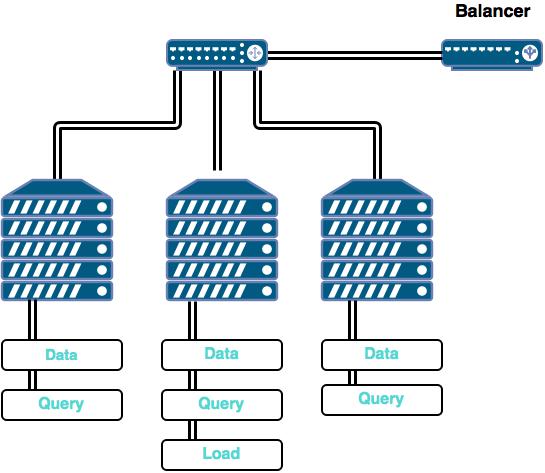
Such deployment is essentially an equivalent of 7 nodes in terms of RAM resources, but still uses CPU and disk resources of only 5 nodes.
Note that even that amount of RAM was not sufficient to run Cascade completely in memory, so the test for scale factor 1000 was run against disk-based configuration of Cascade. The tests for scale factors 100 and 300 were run against in-memory configuration of Cascade.
The benchmark was run on small cluster at Mellanox Technologies Labs,
Mellanox Technologies is a leading supplier of intelligent interconnect solutions for hyper-converged infrastructure. The cluster was connected via Mellanox intelligent 1012 switch.
The benchmark used 5 servers built from commercially off-the shelf parts and open source OS:
| Hardware | Part | Quantity |
|---|---|---|
| Motherboard | SUPERMICRO MBD-X9DRD-7LN4F-O Extended ATX Server | 1 |
| CPU | Intel E5-2670 2.6GHz 20MB Cache 8-Core 115W Processors | 2 |
| Memory | HYNIX HMT31GR7CFR4C-PB 8GB DDR3 | 8 |
| Disk | Micron M500DC 800GB SSD | 1 |
| Network | Mellanox InfiniBand 10Gbs NIC | 2 |
| OS | CentOS Linux 7.1 | 1 |
| Hardware | Part | Quantity |
|---|---|---|
| CPU | Intel i7-5820K 3.3GHz 15 MB Cache 6-Core Processor | 1 |
| Memory | 8GB DDR3 | 8 |
| Disk | Toshiba DT01ACA200 2GB HD | 1 |
| OS | Windows 10 Professional | 1 |
| Scale Factor | Number of nodes |
|---|---|
| 100 (single) | 1 |
| 100 (cluster) | 3 |
| 300 | 4 |
| 1000 | 5 |
For the scale factor 1000 test, two of the nodes were equipped with additional 64 GB of RAM.
Schema design for SSB consists of defining attributes (logical elements of the schema), sources (physical elements of the schema), and finally - relationships and bindings that connect the pieces together.
For each of the four types of attributes, there are appropriate commands:
              CREATE ATTRIBUTE name dataType [WITH properties];
              CREATE ORDERED ATTRIBUTE name dataType [WITH properties];
              CREATE ATTRIBUTE ALIAS name target;
              CREATE COMPOSITE ATTRIBUTE name dataType (components);
              # Measures

              CREATE ATTRIBUTE orderPriority ENUM WITH cardinality=5 values={"1-URGENT", "2-HIGH", "3-MEDIUM", "4-NOT SPECI", "5-LOW"};

              CREATE ATTRIBUTE shipPriority ENUM WITH values={"0"};
              CREATE ORDERED ATTRIBUTE extendedPrice DOUBLE;
              CREATE ORDERED ATTRIBUTE orderTotalPrice DOUBLE;
              CREATE ORDERED ATTRIBUTE revenue INTEGER;
              CREATE ORDERED ATTRIBUTE supplyCost INTEGER;
              CREATE ORDERED ATTRIBUTE tax DOUBLE;
              CREATE ATTRIBUTE shipMode ENUM WITH cardinality=7 values={"TRUCK", "FOB", "SHIP", "AIR", "RAIL", "MAIL", "REG AIR"};
              CREATE ORDERED ATTRIBUTE quantity INTEGER WITH min=0 max=50;
              CREATE ORDERED ATTRIBUTE discount INTEGER WITH min=0 max=10;


              # Part attributes

              CREATE ORDERED ATTRIBUTE partKey INTEGER WITH min=1 max=2000000;
              CREATE ATTRIBUTE partName ENUM;
              CREATE ATTRIBUTE mfgr ENUM WITH cardinality=5;
              CREATE ATTRIBUTE category ENUM WITH cardinality=25;
              CREATE ORDERED ATTRIBUTE brand ENUM WITH prefixTransformer="MFGR#" min="MFGR#0" max="MFGR#9999";
              CREATE ATTRIBUTE color ENUM WITH cardinality=94;
              CREATE ATTRIBUTE type ENUM WITH cardinality=150;
              CREATE ORDERED ATTRIBUTE size INTEGER WITH min=1 max=50;
              CREATE ATTRIBUTE container ENUM WITH cardinality=40;


              # Contact attributes

              CREATE ATTRIBUTE address ENUM;
              CREATE ATTRIBUTE city ENUM WITH cardinality=250;
              CREATE ATTRIBUTE nation ENUM WITH cardinality=25;
              CREATE ATTRIBUTE region ENUM WITH cardinality=5;
              CREATE ATTRIBUTE phone ENUM;


              # Supplier attributes

              CREATE ATTRIBUTE supplierName ENUM WITH cardinality=2000000;
              CREATE ATTRIBUTE ALIAS supplierAddress address;
              CREATE ATTRIBUTE ALIAS supplierCity city;
              CREATE ATTRIBUTE ALIAS supplierNation nation;
              CREATE ATTRIBUTE ALIAS supplierRegion region;
              CREATE ATTRIBUTE ALIAS supplierPhone phone;


              # Customer attributes

              CREATE ATTRIBUTE customerName ENUM WITH cardinality=30000000;
              CREATE ATTRIBUTE ALIAS customerAddress address;
              CREATE ATTRIBUTE ALIAS customerCity city;
              CREATE ATTRIBUTE ALIAS customerNation nation;
              CREATE ATTRIBUTE ALIAS customerRegion region;
              CREATE ATTRIBUTE ALIAS customerPhone phone;
              CREATE ATTRIBUTE marketSegment ENUM;


              # Date attributes

              CREATE ATTRIBUTE date ENUM;
              CREATE ATTRIBUTE dayOfWeek ENUM WITH cardinality=7;
              CREATE ATTRIBUTE month ENUM WITH cardinality=12;
              CREATE ORDERED ATTRIBUTE year INTEGER WITH min=1991 max=1998;
              CREATE ATTRIBUTE yearMonth ENUM;
              CREATE ORDERED ATTRIBUTE dayNumInWeek INTEGER WITH min=1 max=7;
              CREATE ORDERED ATTRIBUTE dayNumInMonth INTEGER WITH min=1 max=31;
              CREATE ORDERED ATTRIBUTE dayNumInYear INTEGER WITH min=1 max=366;
              CREATE ORDERED ATTRIBUTE monthNumInYear INTEGER WITH min=1 max=12;
              CREATE COMPOSITE ATTRIBUTE yearMonthNum INTEGER  (monthNumInYear, year);
              SET BINDINGS yearMonthNum  year="yearMonthNum/100"  monthNumInYear="yearMonthNum%100"  yearMonthNum="year*100+monthNumInYear";
              CREATE ORDERED ATTRIBUTE weekNumInYear INTEGER WITH min=1 max=53;
              CREATE ATTRIBUTE sellingSeason ENUM;
              CREATE ORDERED ATTRIBUTE lastDayInWeekFl INTEGER WITH min=0 max=1;
              CREATE ORDERED ATTRIBUTE lastDayInMonthFl INTEGER WITH min=0 max=1;
              CREATE ORDERED ATTRIBUTE holidayFl INTEGER WITH min=0 max=1;
              CREATE ORDERED ATTRIBUTE weekdayFl INTEGER WITH min=0 max=1;

              COMMIT;
Sources are used to describe contents of the files generated by the SSB data generator tool. Source definition resembles typical DDL, but includes additional properties.
              # Shell script for creating SSBM sources for SF = 1000

              #######
              # Parts (partial urls ok)
              #######

              CREATE SOURCE part1
                  WITH
                  connector=file:delimited
                  delimiter="|"
                  skipHeader=false
                  url=cascade-benchmark/ssb/mysql/ssb1000/part.txt
                  columns= (
                      partKey INTEGER,
                      partName ENUM,
                      mfgr ENUM,
                      category ENUM,
                      brand ENUM,
                      color ENUM,
                      type ENUM,
                      size INTEGER,
                      container ENUM
                  );


              ###########
              # Suppliers (partial urls ok)
              ###########

              CREATE SOURCE supplier1
                  WITH
                  connector=file:delimited
                  delimiter="|"
                  skipHeader=false
                  url=cascade-benchmark/ssb/mysql/ssb1000/supplier.txt
                  columns= (
                      supplierKey INTEGER,
                      supplierName ENUM,
                      supplierAddress ENUM,
                      supplierCity ENUM,
                      supplierNation ENUM,
                      supplierRegion ENUM,
                      supplierPhone ENUM
                  );


              ###########
              # Customers (partial urls ok)
              ###########

              CREATE SOURCE customer1
                  WITH
                  connector=file:delimited
                  delimiter="|"
                  skipHeader=false
                  url=cascade-benchmark/ssb/mysql/ssb1000/customer.txt
                  columns= (
                      customerKey INTEGER,
                      customerName ENUM,
                      customerAddress ENUM,
                      customerCity ENUM,
                      customerNation ENUM,
                      customerRegion ENUM,
                      customerPhone ENUM,
                      marketSegment ENUM
                  );


              #######
              # Dates (partial urls ok)
              #######

              CREATE SOURCE date1
                  WITH
                  connector=file:delimited
                  delimiter="|"
                  skipHeader=false
                  url=cascade-benchmark/ssb/mysql/ssb1000/date.txt
                  columns= (
                      dateKey INTEGER,
                      date ENUM,
                      dayOfWeek ENUM,
                      month ENUM,
                      year INTEGER,
                      yearMonthNum INTEGER,
                      yearMonth ENUM,
                      dayNumInWeek INTEGER,
                      dayNumInMonth INTEGER,
                      dayNumInYear INTEGER,
                      monthNumInYear INTEGER,
                      weekNumInYear INTEGER,
                      sellingSeason ENUM,
                      lastDayInWeekFl INTEGER,
                      lastDayInMonthFl INTEGER,
                      holidayFl INTEGER,
                      weekdayFl INTEGER
                   );


              ####
              # FT (partial urls ok)
              ####

              CREATE SOURCE lineorder1
                  WITH
                  connector=file:delimited
                  delimiter="|"
                  skipHeader=false
                  url=cascade-benchmark/ssb/mysql/ssb1000/lineorder/*.txt
                  columns= (
                      orderKey INTEGER,
                      lineNumber INTEGER,
                      customerKey INTEGER,
                      partKey INTEGER,
                      supplierKey INTEGER,
                      orderDate INTEGER,
                      orderPriority ENUM,
                      shipPriority ENUM,
                      quantity INTEGER,
                      extendedPrice DOUBLE,
                      orderTotalPrice DOUBLE,
                      discount INTEGER,
                      revenue INTEGER,
                      supplyCost INTEGER,
                      tax DOUBLE,
                      commitDate INTEGER,
                      shipMode ENUM
                  );

              COMMIT;
File sources defined above need to be combined into a schema created around the fact table (FTSource). Appropriate relationships are created in the context of each source if they have bindings to that source. Those that go across sources are created within the schema itself.
The following constructs are used below:
              CREATE DEPENDENCY first -> second IN context;
              CREATE JOIN first ~ second IN context;
              CREATE EQUIVALENCE first ~ second IN context;
              CREATE ASSOCIATION first ~> second IN context;
              CREATE BINDING variable -> expression IN context;
Here first/second can be a Column, an Attribute or an array or attributes (for "star rule"), and Expression can be a Column or Attribute or an expression in terms of Columns and Attributes.
              # Shell script for creating SSBM SCHEMA and Rules for SF = 1000

              ## Create schema

              CREATE SCHEMA lineorder1_schema FROM SOURCE lineorder1;

              ## Add star dependency

              CREATE DEPENDENCY
                 {partKey, date, customerName, supplierName, quantity, discount} ->
                 {orderPriority, shipPriority, extendedPrice, orderTotalPrice, revenue, supplyCost, tax, shipMode}
              IN   lineorder1_schema;

              ## Add bindings

              CREATE  BINDING orderPriority   ->  lineorder1_schema.orderPriority     IN  lineorder1_schema;
              CREATE  BINDING shipPriority    ->  lineorder1_schema.shipPriority      IN  lineorder1_schema;
              CREATE  BINDING extendedPrice   ->  lineorder1_schema.extendedPrice     IN  lineorder1_schema;
              CREATE  BINDING orderTotalPrice ->  lineorder1_schema.orderTotalPrice   IN  lineorder1_schema;
              CREATE  BINDING revenue         ->  lineorder1_schema.revenue           IN  lineorder1_schema;
              CREATE  BINDING supplyCost      ->  lineorder1_schema.supplyCost        IN  lineorder1_schema;
              CREATE  BINDING tax             ->  lineorder1_schema.tax               IN  lineorder1_schema;
              CREATE  BINDING shipMode        ->  lineorder1_schema.shipMode          IN  lineorder1_schema;


              ##  Add sources and bindings for dimensions within relevant sources

              CREATE  BINDING quantity  ->  lineorder1_schema.quantity   IN   lineorder1_schema;
              CREATE  BINDING discount  ->  lineorder1_schema.discount   IN   lineorder1_schema;

              CREATE  BINDING partKey     ->  part1.partKey   IN  part1;
              CREATE  BINDING mfgr        ->  part1.mfgr      IN  part1;
              CREATE  BINDING brand       ->  part1.brand     IN  part1;
              CREATE  BINDING category    ->  part1.category  IN  part1;
              ADD SOURCE part1 TO lineorder1_schema;

              CREATE  BINDING supplierName    ->  supplier1.supplierName      IN  supplier1;
              CREATE  BINDING supplierRegion  ->  supplier1.supplierRegion    IN  supplier1;
              CREATE  BINDING supplierNation  ->  supplier1.supplierNation    IN  supplier1;
              CREATE  BINDING supplierCity    ->  supplier1.supplierCity      IN  supplier1;
              ADD SOURCE supplier1 TO lineorder1_schema;

              CREATE  BINDING customerName    ->  customer1.customerName      IN  customer1;
              CREATE  BINDING customerRegion  ->  customer1.customerRegion    IN  customer1;
              CREATE  BINDING customerNation  ->  customer1.customerNation    IN  customer1;
              CREATE  BINDING customerCity    ->  customer1.customerCity      IN  customer1;
              ADD SOURCE customer1 TO lineorder1_schema;

              CREATE  BINDING date            ->  date1.date              IN  date1;
              CREATE  BINDING year            ->  date1.year              IN  date1;
              CREATE  BINDING yearMonth       ->  date1.yearMonth         IN  date1;
              CREATE  BINDING yearMonthNum    ->  date1.yearMonthNum      IN  date1;
              CREATE  BINDING weekNumInYear   ->  date1.weekNumInYear     IN  date1;
              CREATE  BINDING monthNumInYear  ->  date1.monthNumInYear    IN  date1;
              ADD SOURCE date1 TO lineorder1_schema;


              ## Joins
              CREATE JOIN lineorder1_schema.partKey       ~   part1.partKey           IN  lineorder1_schema;
              CREATE JOIN lineorder1_schema.supplierKey   ~   supplier1.supplierKey   IN  lineorder1_schema;
              CREATE JOIN lineorder1_schema.customerKey   ~   customer1.customerKey   IN  lineorder1_schema;
              CREATE JOIN lineorder1_schema.orderDate     ~   date1.dateKey           IN  lineorder1_schema;


              ##  Add scalar dependencies

              CREATE DEPENDENCY   partKey     ->  brand       IN    part1;
              CREATE DEPENDENCY   brand       ->  category    IN    part1;
              CREATE DEPENDENCY   category    ->  mfgr        IN    part1;

              CREATE DEPENDENCY   supplierName  ->  supplierCity  IN    supplier1;
              CREATE DEPENDENCY   supplierCity  ->  supplierNation  IN    supplier1;
              CREATE DEPENDENCY   supplierNation  ->  supplierRegion  IN    supplier1;
              CREATE EQUIVALENCE  supplier1.supplierKey   ~   supplierName    IN supplier1;

              CREATE DEPENDENCY   customerName  ->  customerCity  IN    customer1;
              CREATE DEPENDENCY   customerCity  ->  customerNation  IN    customer1;
              CREATE DEPENDENCY   customerNation  ->  customerRegion  IN    customer1;
              CREATE EQUIVALENCE  customer1.customerKey   ~   customerName    IN customer1;


              CREATE DEPENDENCY   date  ->  yearMonthNum  IN    date1;
              CREATE DEPENDENCY   date  ->  weekNumInYear  IN    date1;
              CREATE ATTRIBUTE EQUIVALENCE yearMonthNum  ~ yearMonth IN  date1;

              CREATE EQUIVALENCE  date1.dateKey           ~   date            IN date1;

              CREATE STAR lineorder1000 FROM lineorder1_schema;

              COMMIT;
This completes schema definitions for Star Schema Benchmark
Data load for SSB was performed in two steps: create encoders and deploy star.
              # Shell script for creating SSBM ENCODERS for SF = 1000

              DEPLOY ENCODERS FOR lineorder1000;

              COMMIT;

              # Shell script for DEPLOY SSBM STAR(s) for SF = 1000

              DEPLOY STAR lineorder1000
                  WITH
                  dataNodes = {localhost}
                  intendedCardinality = 6000000000
                  protocol = cascade:remote
                  partitionCount = 160
                  partitionKind = ROUND_ROBIN
              COMMIT;
Consider a business process in which customers buy certain products for certain stores. The business owner keeps track of the sales noting the time of sale, the amount and the cost. That is what we want to model in "Hello, world!" case.
Imagine that there is a CSV file with 1,000,000 sales records, and we want to ask some analytic questions regarding that data. We will play both the role of business expert and data expert for this exercise
We will use Cascade Shell scripts to set everything up. Here are the steps:
              CREATE ATTRIBUTE customer ENUM;
              CREATE ATTRIBUTE product ENUM;
              CREATE ATTRIBUTE store ENUM;
              CREATE ORDERED ATTRIBUTE time TIMESTAMP;
              CREATE ORDERED ATTRIBUTE sales INTEGER;
              CREATE ORDERED ATTRIBUTE cost INTEGER;
              CREATE SOURCE salesFile
                  WITH
                  connector=file:delimited
                  delimiter="|"
                  skipHeader=false
                  url=sources/sales.txt
                  columns= (
                      customer ENUM,
                      product ENUM,
                      store ENUM,
                      time TIMESTAMP,
                      sales INTEGER,
                      cost INTEGER);
              CREATE SCHEMA starSchema FROM SOURCE salesFile;

              CREATE DEPENDENCY (customer, product, store, time) -> (sales, cost) IN starSchema;
              # Add bindings for attributes to identically named columns
              CREATE BINDING customer -> starSchema.customer IN starSchema;
              CREATE BINDING product -> starSchema.product IN starSchema;
              CREATE BINDING store -> starSchema.store IN starSchema;
              CREATE BINDING time -> starSchema.time IN starSchema;
              CREATE BINDING sales -> starSchema.sales IN starSchema;
              CREATE BINDING cost -> starSchema.cost IN starSchema;
              CREATE STAR salesStar FROM starSchema;
              DEPLOY ENCODERS FOR salesStar;
              COMMIT;

              DEPLOY STAR salesStar
                  WITH
                  intendedCardinality = 1000000
                  protocol = cascade
                  partitionCount = 4
                  partitionKind = ROUND_ROBIN
              COMMIT;
Run the script, and we are done. We are ready to submit queries to Cascade. This can be done from Cascade Shell or from any UI tool that supports JDBC or ODBC sources. Note that both the context "salesFile" and the context "salesStar" are available for querying. Queries will return the same results, but there will be a big difference in response times.
Example of a query is
              select customer, sum(sales-cost) as profit
              from salesStar
              where product='Coke' and store='Palo Alto'
              group by customer